R Notebook
Last updated: 2019-05-14
Checks: 6 0
Knit directory: 10x-adipocyte-analysis/
This reproducible R Markdown analysis was created with workflowr (version 1.2.0). The Report tab describes the reproducibility checks that were applied when the results were created. The Past versions tab lists the development history.
Great! Since the R Markdown file has been committed to the Git repository, you know the exact version of the code that produced these results.
Great job! The global environment was empty. Objects defined in the global environment can affect the analysis in your R Markdown file in unknown ways. For reproduciblity it’s best to always run the code in an empty environment.
The command set.seed(20181026) was run prior to running the code in the R Markdown file. Setting a seed ensures that any results that rely on randomness, e.g. subsampling or permutations, are reproducible.
Great job! Recording the operating system, R version, and package versions is critical for reproducibility.
Nice! There were no cached chunks for this analysis, so you can be confident that you successfully produced the results during this run.
Great! You are using Git for version control. Tracking code development and connecting the code version to the results is critical for reproducibility. The version displayed above was the version of the Git repository at the time these results were generated.
Note that you need to be careful to ensure that all relevant files for the analysis have been committed to Git prior to generating the results (you can use wflow_publish or wflow_git_commit). workflowr only checks the R Markdown file, but you know if there are other scripts or data files that it depends on. Below is the status of the Git repository when the results were generated:
Ignored files:
    Ignored:    code/.Rhistory
    Ignored:    figures/
    Ignored:    output/bulk_analysis/
    Ignored:    output/demuxlet/
    Ignored:    output/markergenes/
    Ignored:    output/monocle/
    Ignored:    output/seurat_objects/
    Ignored:    output/velocyto/
    Ignored:    output/wgcna/
    Ignored:    tables/

Untracked files:
    Untracked:  .rstudio_old10/
    Untracked:  10x-adipocyte-analysis-copy.Rproj
    Untracked:  analysis/.ipynb_checkpoints/velocyto_notebook_180831-checkpoint.ipynb
    Untracked:  analysis/10-180831-monocle-per-depot.Rmd
    Untracked:  analysis/10x-180831-BEAM-heatmap.Rmd
    Untracked:  analysis/10x-180831-pseudotime.Rmd
    Untracked:  code/BEAM-heatmaps.R
    Untracked:  code/BEAM_gsea.R
    Untracked:  code/colors.R

Unstaged changes:
    Deleted:    10x-adipocyte-analysis.Rproj
    Modified:   analysis/10x-180504-DEGs-depots.Rmd
    Modified:   analysis/10x-180504-alignment.Rmd
    Modified:   analysis/10x-180504-depot-markers.Rmd
    Modified:   analysis/10x-180831-BATLAS.Rmd
    Modified:   analysis/10x-180831-TF_analysis.Rmd
    Modified:   analysis/10x-180831-beamGOplot.Rmd
    Modified:   analysis/10x-180831-colors.Rmd
    Modified:   analysis/10x-180831-figures.Rmd
    Modified:   analysis/10x-180831-general-analysis.Rmd
    Modified:   analysis/10x-180831-supplementary_figures.Rmd
    Modified:   analysis/velocyto_notebook_180504.ipynb
    Modified:   analysis/velocyto_notebook_180831.ipynb
    Deleted:    code/REMOVE/find-brown-sample-markers-180504-REMOVE.R
    Deleted:    code/REMOVE/find-white-sample-markers-180504-REMOVE.R
    Deleted:    code/REMOVE/get-genes-monocle-180831-REMOVE.R
    Modified:   code/compute-genelists-monocle-depots.R
    Modified:   code/find-depot-markers-180504.R
    Modified:   code/find-markers.R
    Modified:   code/preprocess-data.R
    Modified:   code/run-alignment.R
    Modified:   code/run-monocle.R
    Modified:   code/velocyto_preprocess.py
Note that any generated files, e.g. HTML, png, CSS, etc., are not included in this status report because it is ok for generated content to have uncommitted changes.
These are the previous versions of the R Markdown and HTML files. If you’ve configured a remote Git repository (see ?wflow_git_remote), click on the hyperlinks in the table below to view them.
| File | Version | Author | Date | Message |
|---|---|---|---|---|
| Rmd | faf7b78 | Pytrik Folkertsma | 2019-05-14 | Notebook cleanup |
| html | 0abf4f1 | Pytrik Folkertsma | 2019-05-13 | Build site. |
| Rmd | b2735de | Pytrik Folkertsma | 2019-05-13 | Notebook cleanup |
| html | 7edfe73 | Pytrik Folkertsma | 2019-04-04 | Build site. |
| Rmd | 8e41685 | Pytrik Folkertsma | 2019-04-04 | updated BEAM analysis |
| html | 9ced468 | Pytrik Folkertsma | 2019-04-04 | Build site. |
| Rmd | 7ef9f33 | Pytrik Folkertsma | 2019-04-04 | updated BEAM analysis |
| html | b3cc370 | Pytrik Folkertsma | 2019-04-04 | Build site. |
| Rmd | 859bb51 | Pytrik Folkertsma | 2019-04-04 | updated BEAM analysis |
| html | 13994df | Pytrik Folkertsma | 2019-04-03 | Build site. |
| Rmd | ddbc7bc | Pytrik Folkertsma | 2019-04-03 | new heatmaps |
| html | 4d92211 | Pytrik Folkertsma | 2019-04-03 | Build site. |
| Rmd | 7f0e856 | Pytrik Folkertsma | 2019-04-03 | new heatmaps |
| html | b064e18 | Pytrik Folkertsma | 2019-04-03 | Build site. |
| Rmd | d828f8b | Pytrik Folkertsma | 2019-04-03 | updated monocle notebook |
| Rmd | 03050a1 | Pytrik Folkertsma | 2019-03-28 | analysis updates |
| html | 221a47f | Pytrik Folkertsma | 2019-01-04 | docs |
| Rmd | ab801ec | Pytrik Folkertsma | 2019-01-04 | updated notebooks |
library(Seurat)
library(monocle)
library(pheatmap)
library(knitr)
library(gtools)
library(dplyr)
library(kableExtra)
source('code/colors.R')
seurobj <- readRDS('output/seurat_objects/180831/10x-180831')
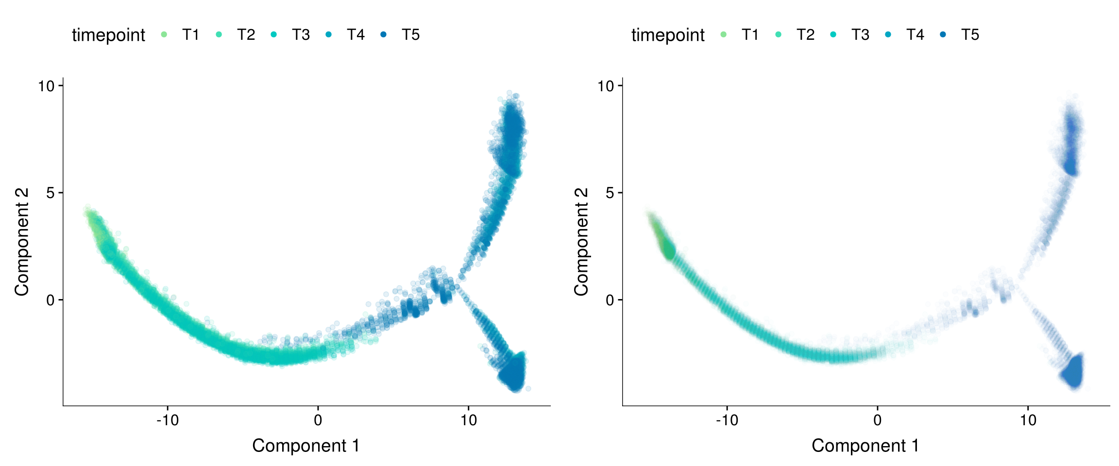
cds <- readRDS('output/monocle/180831/10x-180831-monocle-monocle_genelist_T1T2T3_T4T5_res.1.5')Trajectory plots
fig <- plot_grid(ncol=1,
  plot_cell_trajectory(cds, color_by='timepoint') + scale_color_manual(values=colors.timepoints, name = "Timepoint"),
  plot_cell_trajectory(cds, color_by='Pseudotime'),
  plot_cell_trajectory(cds, color_by='State'),
  plot_cell_trajectory(cds, color_by = "State") + scale_color_manual(values=colors.states, name = "State"))

fig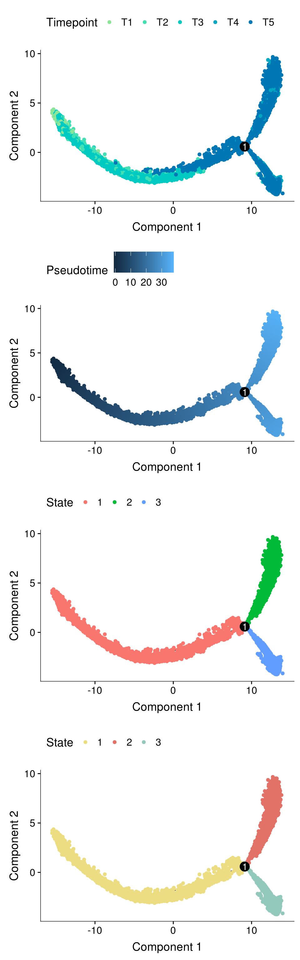
plot_cell_trajectory(cds, color_by='depot') + scale_color_manual(values=colors.depots, name = 'Depots')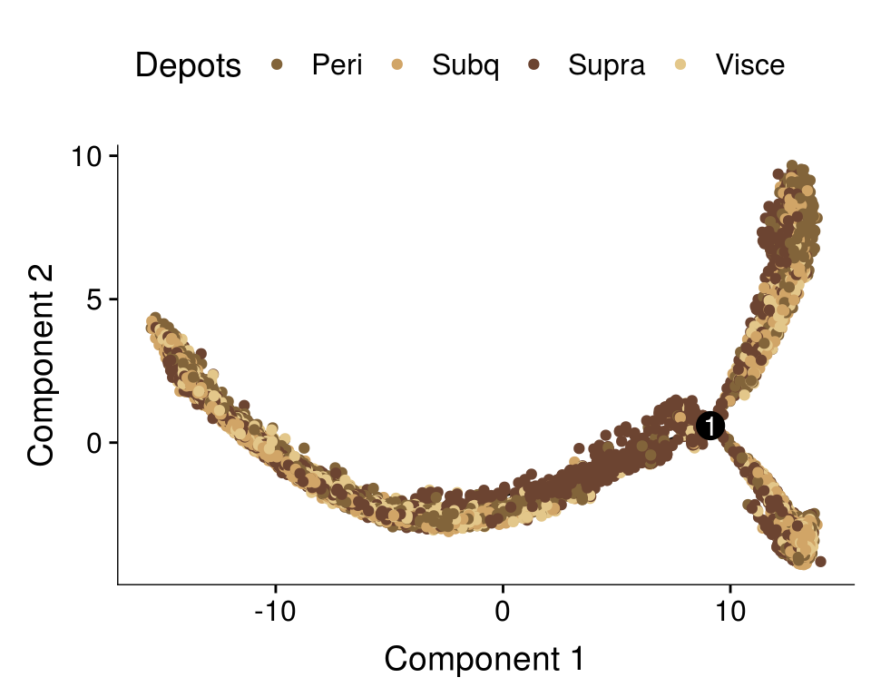
plot_cell_trajectory(cds, color_by='type') + scale_color_manual(values=colors.type, name = "Type")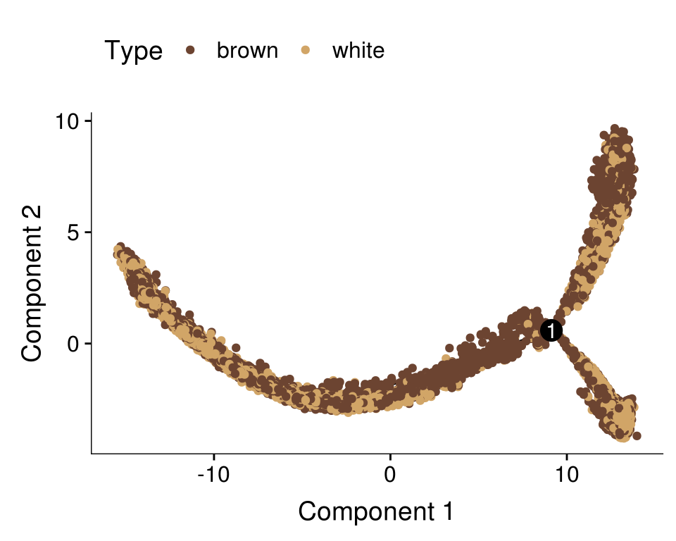
Predicted labels by Monocle vs fat type.
#seurobj <- AddMetaData(seurobj, pData(cds)['State'])
p <- plot_grid(
  TSNEPlot(seurobj, group.by='State', pt.size=0.1, colors.use=colors.states, return.plot=T),
  TSNEPlot(seurobj, group.by='type', pt.size=0.1, colors.use=colors.type, return.plot=T),
  labels=c('Predicted by Monocle', 'Type')
)
p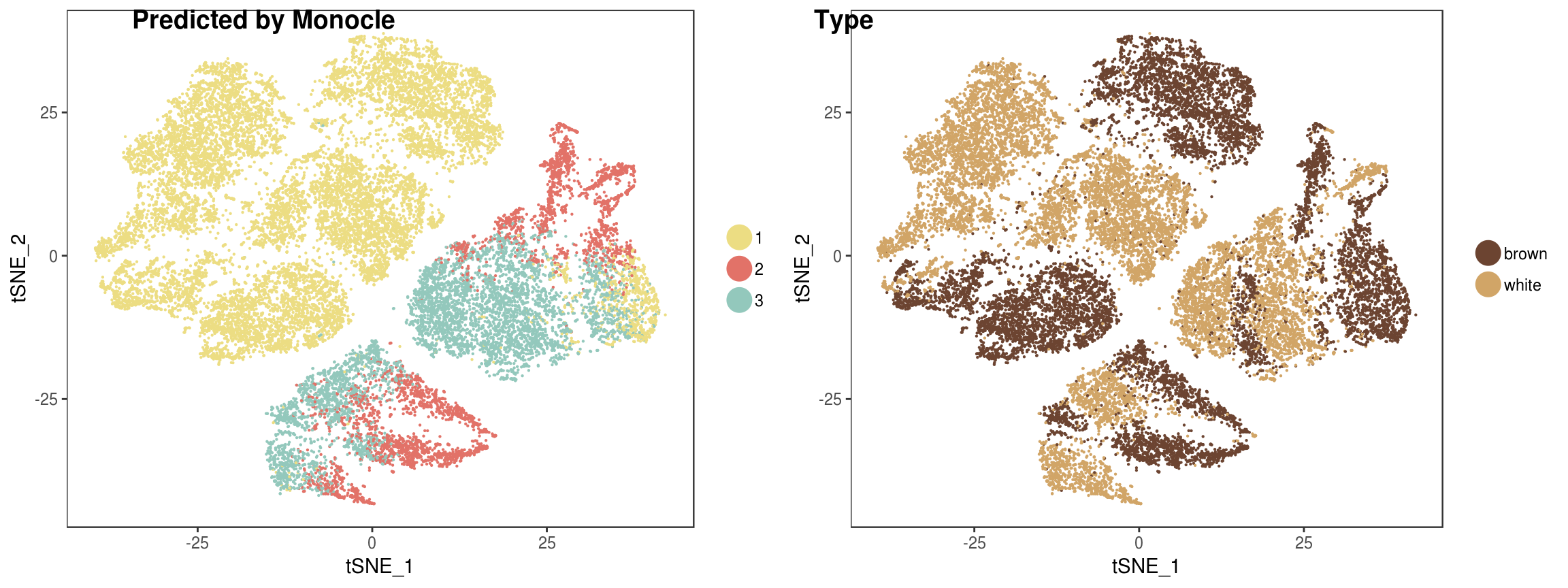
Depots and timepoints in Seurat tSNE.
p <- plot_grid(
  TSNEPlot(seurobj, group.by='depot', pt.size=0.1, colors.use=colors.depots, return.plot=T),
  TSNEPlot(seurobj, group.by='timepoint', pt.size=0.1, colors.use=colors.timepoints, return.plot=T),
  ncol=2
)
p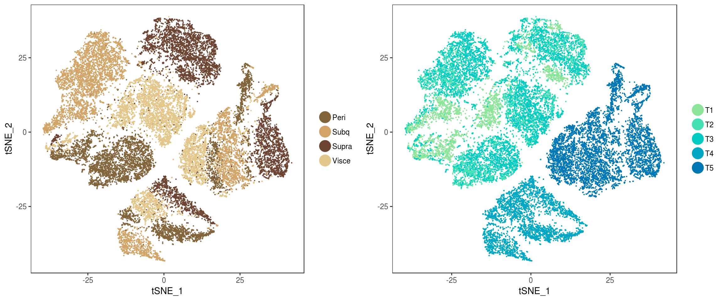
Trajectory transparency.
plot_grid(
  plot_cell_trajectory(cds, color_by = "timepoint") + geom_point(color='white', size=5) + geom_point(aes(colour=timepoint), alpha=0.1) + scale_color_manual(values=colors.timepoints),
  plot_cell_trajectory(cds, color_by = "timepoint") + geom_point(color='white', size=5) + geom_point(aes(colour=timepoint), alpha=0.01) + scale_color_manual(values=colors.timepoints),
  ncol=2
)
| Version | Author | Date |
|---|---|---|
| b064e18 | Pytrik Folkertsma | 2019-04-03 |
Pseudotime deciles
TSNEPlot(seurobj, group.by='branch_high_res', colors.use=colors.deciles.gradient, pt.size=0.5)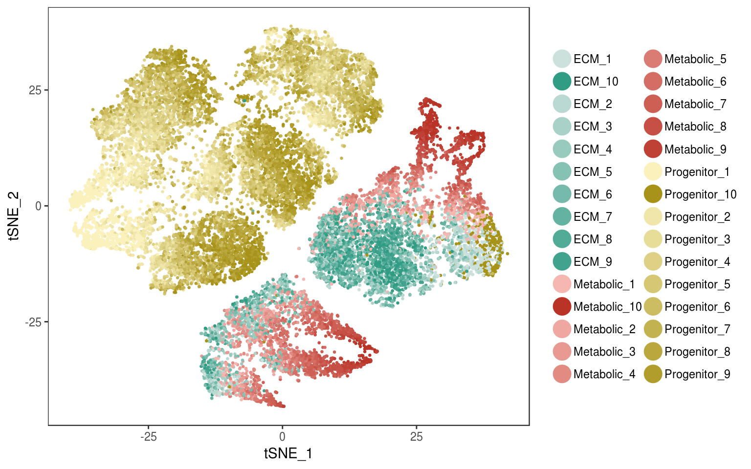
| Version | Author | Date |
|---|---|---|
| b064e18 | Pytrik Folkertsma | 2019-04-03 |
#save_plot('../figures/figures_paper/supplementary_figures/10x-180831_tsne-deciles-pseudotime.pdf', p, base_height=5, base_width=8)Ratio’s brown/white in branches
Ratio’s white/brown and depots per branch.
get_ratios <- function(col1, col2){
  states <- unique(seurobj@meta.data[,col1])
  values <- unique(seurobj@meta.data[,col2])
  df <- as.data.frame(matrix(ncol=length(values)+1, nrow=length(states)))
  colnames(df) <- c('n', values)
  rownames(df) <- states
  for (state in states){
    n_state = length(which(seurobj@meta.data[col1] == state))
    df[state, 'n'] <- n_state
    #print(paste('N cells', col1, state, ':', n_state))
    for (value in values){
        n_state_value <- length(which(seurobj@meta.data[col1] == state & seurobj@meta.data[col2] == value))
        perc_state_value <- n_state_value / n_state
        df[state, value] <- round(perc_state_value, 2)
        #print(paste('Ratio', value, 'in', state, ': ', round(perc_state_value, 2)))
    }
  }
  return(df)
}
states.depots <- get_ratios('State.labels', 'depot')
depots.states <- get_ratios('depot', 'State.labels')
#write.table(states.depots, '../tables/tables_paper/supplementary_tables/10x-180831-ratios-branches-depots.tsv', sep='\t', quote=F, col.names=NA)
#write.table(depots.states, '../tables/tables_paper/supplementary_tables/10x-180831-ratios-depots-branches.tsv', sep='\t', quote=F, col.names=NA)
states.depots n Peri Subq Visce Supra
P 14353 0.23 0.26 0.25 0.26
L 5476 0.17 0.32 0.36 0.16
U 3599 0.39 0.23 0.11 0.27depots.states n P L U
Peri 5599 0.59 0.16 0.25
Subq 6269 0.59 0.28 0.13
Visce 5986 0.60 0.33 0.07
Supra 5574 0.67 0.16 0.18states.types <- get_ratios('State.labels', 'type')
types.states <- get_ratios('type', 'State.labels')
#write.table(states.types, '../tables/tables_paper/supplementary_tables/10x-180831-ratios-branches-types.tsv', sep='\t', quote=F, col.names=NA)
#write.table(types.states, '../tables/tables_paper/supplementary_tables/10x-180831-ratios-types-branches.tsv', sep='\t', quote=F, col.names=NA)
states.types n brown white
P 14353 0.49 0.51
L 5476 0.33 0.67
U 3599 0.66 0.34types.states n P L U
brown 11173 0.63 0.16 0.21
white 12255 0.60 0.30 0.10BEAM
BEAM takes as input a CellDataSet that’s been ordered with orderCells and the name of a branch point in the trajectory. It returns a table of significance scores for each gene. Genes that score significant are said to be branch-dependent in their expression.
#BEAM_res <- BEAM(cds, branch_point = 1, cores = 10)
load('output/monocle/180831/BEAM_new')
BEAM_res <- BEAM_res[order(BEAM_res$qval),]
BEAM_res <- BEAM_res[,c("gene_short_name", "pval", "qval")]
paste('Significant genes with q-val < 0.05:', length(BEAM_res$qval[BEAM_res$qval < 0.05]))[1] "Significant genes with q-val < 0.05: 8647"paste('Significant genes with q-val < 0.01:', length(BEAM_res$qval[BEAM_res$qval < 0.01]))[1] "Significant genes with q-val < 0.01: 7366"paste('Significant genes with q-val < 0.001:', length(BEAM_res$qval[BEAM_res$qval < 0.001]))[1] "Significant genes with q-val < 0.001: 6250"paste('Significant genes with q-val < 0.0001:', length(BEAM_res$qval[BEAM_res$qval < 0.0001]))[1] "Significant genes with q-val < 0.0001: 5523"paste('Significant genes with q-val < 0.00001:', length(BEAM_res$qval[BEAM_res$qval < 0.00001]))[1] "Significant genes with q-val < 0.00001: 5029"paste('Significant genes with q-val = 0:', length(BEAM_res$qval[BEAM_res$qval == 0]))[1] "Significant genes with q-val = 0: 271"Histograms of p-values and q-values
hist(BEAM_res$pval)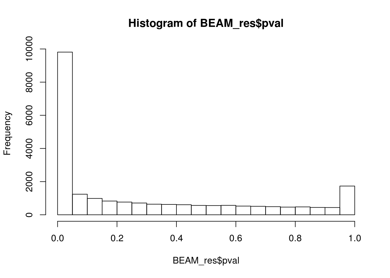
| Version | Author | Date |
|---|---|---|
| 221a47f | Pytrik Folkertsma | 2019-01-04 |
hist(BEAM_res$qval)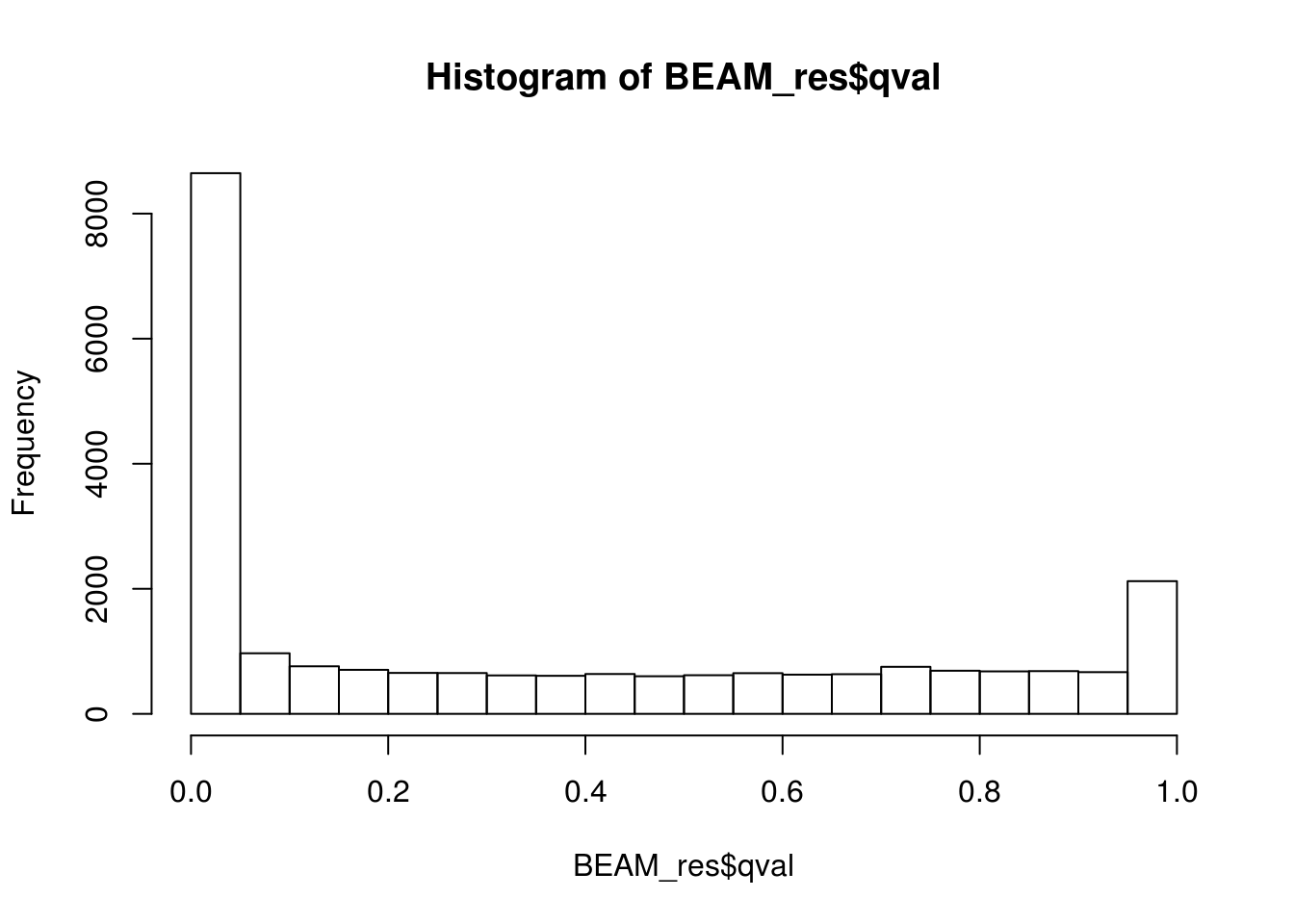
Filtering BEAM results on fold change
matrix <- as.matrix(seurobj@data)
calculateAvgLogFC <- function(gene){
  gene <- as.character(gene)
    state2 <- log1p(mean(expm1(as.numeric(matrix[gene, row.names(seurobj@meta.data)[seurobj@meta.data$State == 2]])))) # first un-log transform. then average. then logp1 again. This is all done to calculate the mean in non-log-space.
  state3 <- log1p(mean(expm1(as.numeric(matrix[gene, row.names(seurobj@meta.data)[seurobj@meta.data$State == 3]]))))
  return(state2-state3)
}

BEAM_signficnat_res <- BEAM_res[BEAM_res$qval < 0.05,]
BEAM_signficnat_res$avgLogFC_State2_State3 <- sapply(BEAM_signficnat_res$gene_short_name, calculateAvgLogFC)
X axis = minimum log fold change.
all <- c()
values <- list()
for (i in seq(0.0, 3, by=0.1)){
  fc <- abs(BEAM_signficnat_res$avgLogFC_State2_State3[abs(BEAM_signficnat_res$avgLogFC_State2_State3) >= i])
  all <- c(all, fc)
  values[toString(i)] <- length(fc)
}
hist(all, breaks=20, probability = F)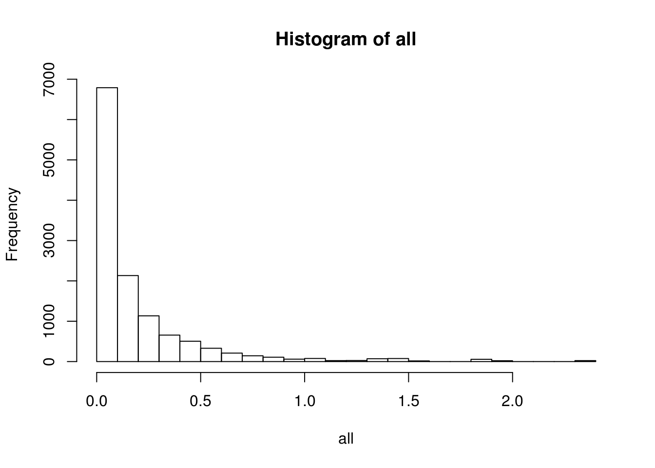
| Version | Author | Date |
|---|---|---|
| b064e18 | Pytrik Folkertsma | 2019-04-03 |
df <- data.frame(min_fold_change=names(values), num_genes=unlist(values))
rownames(df) <- NULL
kable(df) %>%
kable_styling(bootstrap_options = "striped", full_width = F)| min_fold_change | num_genes |
|---|---|
| 0 | 8647 |
| 0.1 | 1857 |
| 0.2 | 791 |
| 0.3 | 413 |
| 0.4 | 249 |
| 0.5 | 148 |
| 0.6 | 93 |
| 0.7 | 63 |
| 0.8 | 45 |
| 0.9 | 33 |
| 1 | 27 |
| 1.1 | 20 |
| 1.2 | 18 |
| 1.3 | 16 |
| 1.4 | 11 |
| 1.5 | 6 |
| 1.6 | 5 |
| 1.7 | 5 |
| 1.8 | 5 |
| 1.9 | 2 |
| 2 | 1 |
| 2.1 | 1 |
| 2.2 | 1 |
| 2.3 | 1 |
| 2.4 | 0 |
| 2.5 | 0 |
| 2.6 | 0 |
| 2.7 | 0 |
| 2.8 | 0 |
| 2.9 | 0 |
| 3 | 0 |
BEAM heatmap
Create heatmap of the significant genes with absolute average logFC > 0.3.
#branched_5_0.3_2 <- plot_genes_branched_heatmap(cds[row.names(subset(BEAM_signficnat_res, abs(avgLogFC_State2_State3) > 0.3))],
#                                         branch_point = 1,
#                                         num_clusters = 5,
#                                         cores = 10,
#                                         show_rownames = T,
#                                       return_heatmap = T,
#                                       branch_labels = c("Upper branch", "Lower branch"),
#                                       branch_colors = colors.states
# )load('output/monocle/180831/heatmaps')You can visualize changes for all the genes that are significantly branch dependent using a special type of heatmap. This heatmap shows changes in both lineages at the same time. It also requires that you choose a branch point to inspect. Columns are points in pseudotime, rows are genes, and the beginning of pseudotime is in the middle of the heatmap. As you read from the middle of the heatmap to the right, you are following one lineage through pseudotime. As you read left, the other. The genes are clustered hierarchically, so you can visualize modules of genes that have similar lineage-dependent expression patterns.\ Below heatmaps with different logFC thresholds and nClusters are shown. For the heatmap in the publication figure, genes were filtered on absolute logFC > 0.3 between U and L branch and clustered in 6 groups.
print_nGene <- function(branched){
  print(paste('Total number of genes:', length(branched$annotation_row$Cluster)))
  for (i in 1:length(unique(branched$annotation_row$Cluster))){
    cluster <- rownames(branched$annotation_row)[branched$annotation_row$Cluster == i]
    print(paste('Nr of genes in cluster ', i, ': ', length(cluster), sep=''))
  }
}
for (name in names(heatmaps)){
cat('\n')
cat(paste('BEAM heatmap:', name))
gridExtra::grid.arrange(heatmaps[[name]]$ph_res$gtable)
cat(print_nGene(heatmaps[[name]]))
cat('\n')
}BEAM heatmap: heatmap_logFC0.3_ncluster3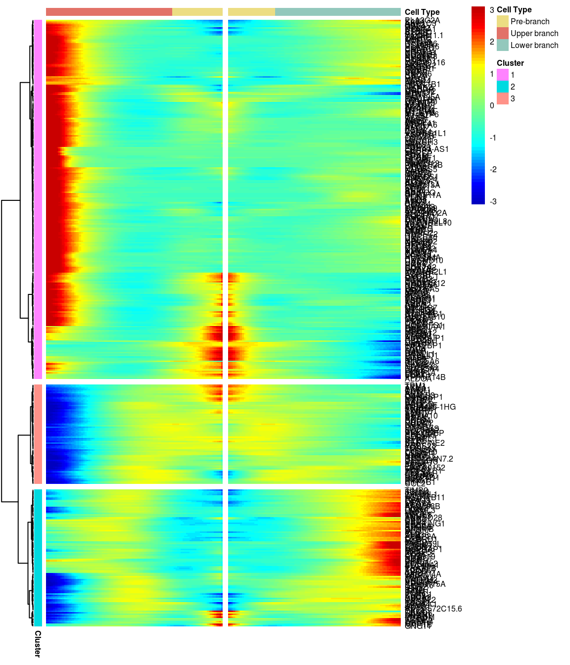 [1] “Total number of genes: 413” [1] “Nr of genes in cluster 1: 249” [1] “Nr of genes in cluster 2: 95” [1] “Nr of genes in cluster 3: 69”
BEAM heatmap: heatmap_logFC0.3_ncluster4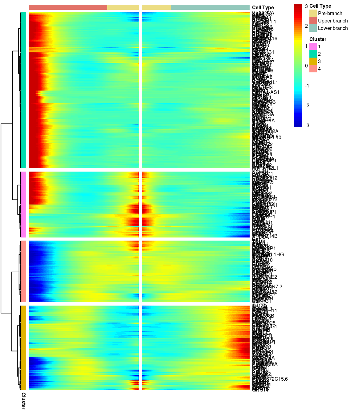 [1] “Total number of genes: 413” [1] “Nr of genes in cluster 1: 74” [1] “Nr of genes in cluster 2: 175” [1] “Nr of genes in cluster 3: 95” [1] “Nr of genes in cluster 4: 69”
BEAM heatmap: heatmap_logFC0.3_ncluster5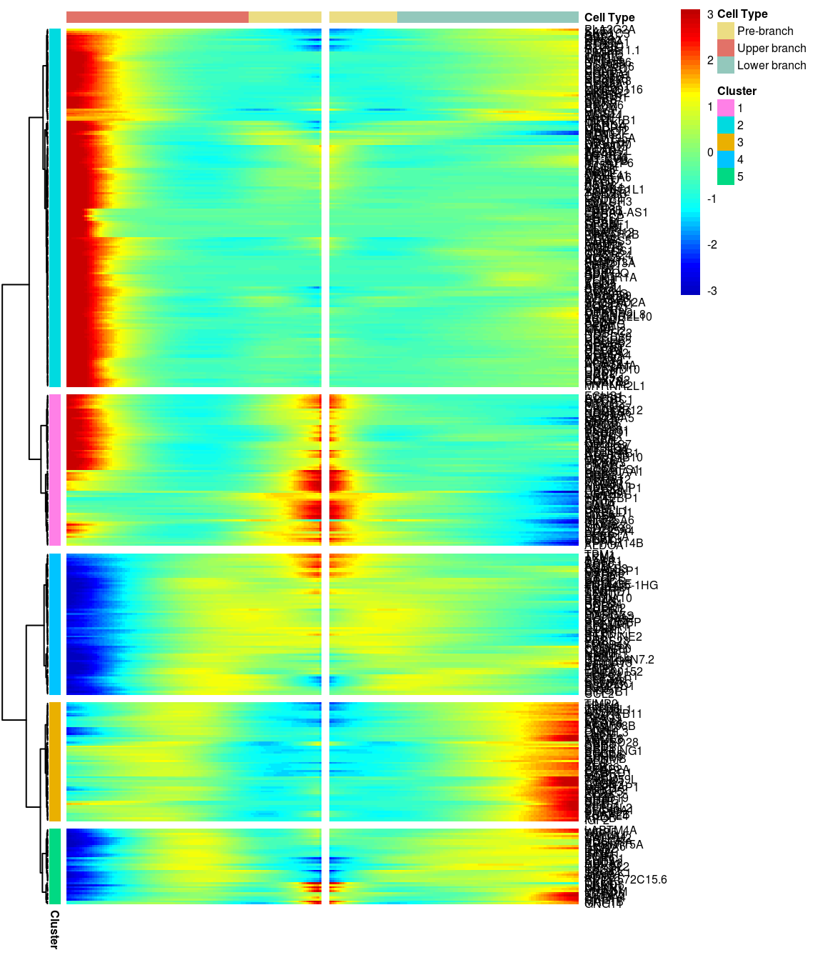 [1] “Total number of genes: 413” [1] “Nr of genes in cluster 1: 74” [1] “Nr of genes in cluster 2: 175” [1] “Nr of genes in cluster 3: 58” [1] “Nr of genes in cluster 4: 69” [1] “Nr of genes in cluster 5: 37”
BEAM heatmap: heatmap_logFC0.3_ncluster6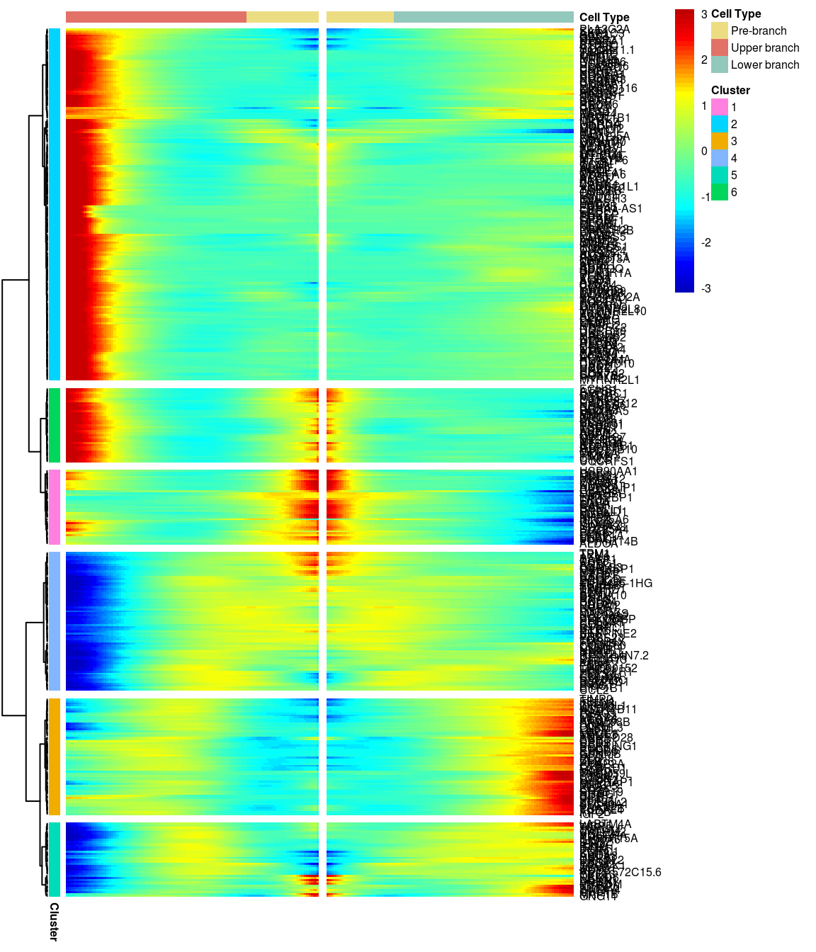 [1] “Total number of genes: 413” [1] “Nr of genes in cluster 1: 37” [1] “Nr of genes in cluster 2: 175” [1] “Nr of genes in cluster 3: 58” [1] “Nr of genes in cluster 4: 69” [1] “Nr of genes in cluster 5: 37” [1] “Nr of genes in cluster 6: 37”
BEAM heatmap: heatmap_logFC0.3_ncluster7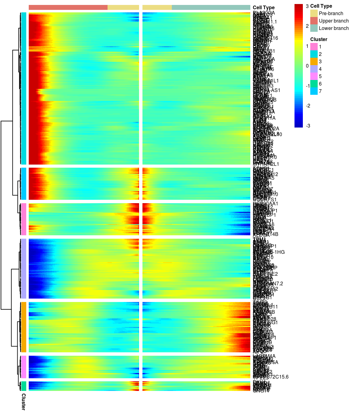 [1] “Total number of genes: 413” [1] “Nr of genes in cluster 1: 37” [1] “Nr of genes in cluster 2: 175” [1] “Nr of genes in cluster 3: 58” [1] “Nr of genes in cluster 4: 69” [1] “Nr of genes in cluster 5: 26” [1] “Nr of genes in cluster 6: 11” [1] “Nr of genes in cluster 7: 37”
BEAM heatmap: heatmap_logFC0.3_ncluster8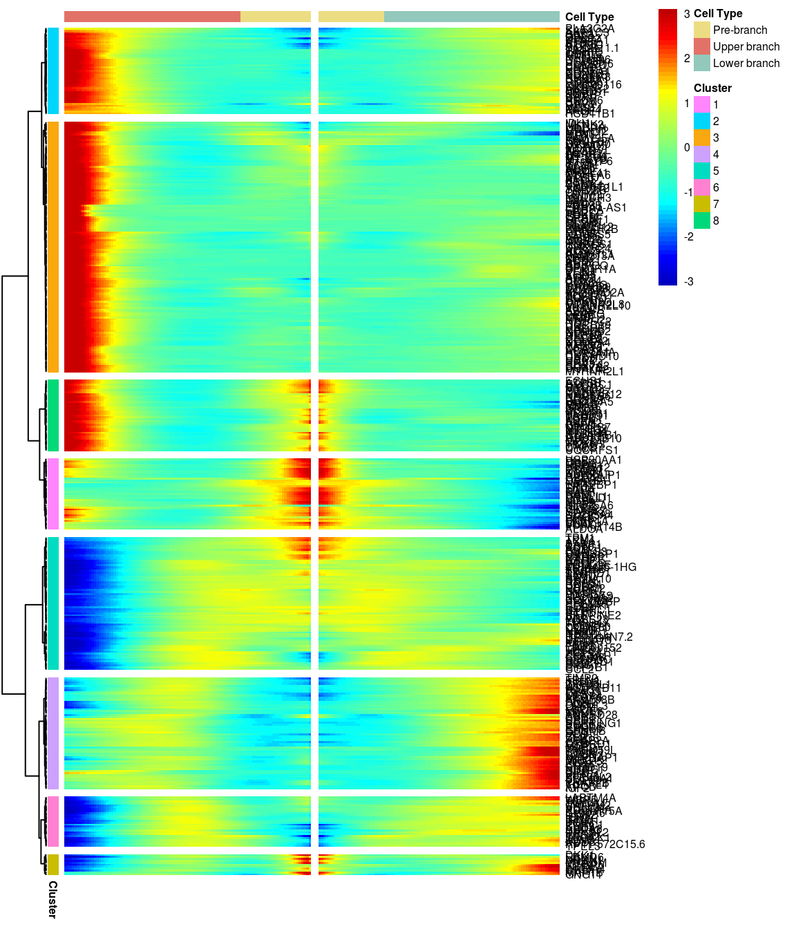 [1] “Total number of genes: 413” [1] “Nr of genes in cluster 1: 37” [1] “Nr of genes in cluster 2: 45” [1] “Nr of genes in cluster 3: 130” [1] “Nr of genes in cluster 4: 58” [1] “Nr of genes in cluster 5: 69” [1] “Nr of genes in cluster 6: 26” [1] “Nr of genes in cluster 7: 11” [1] “Nr of genes in cluster 8: 37”
BEAM heatmap: heatmap_logFC0.4_ncluster3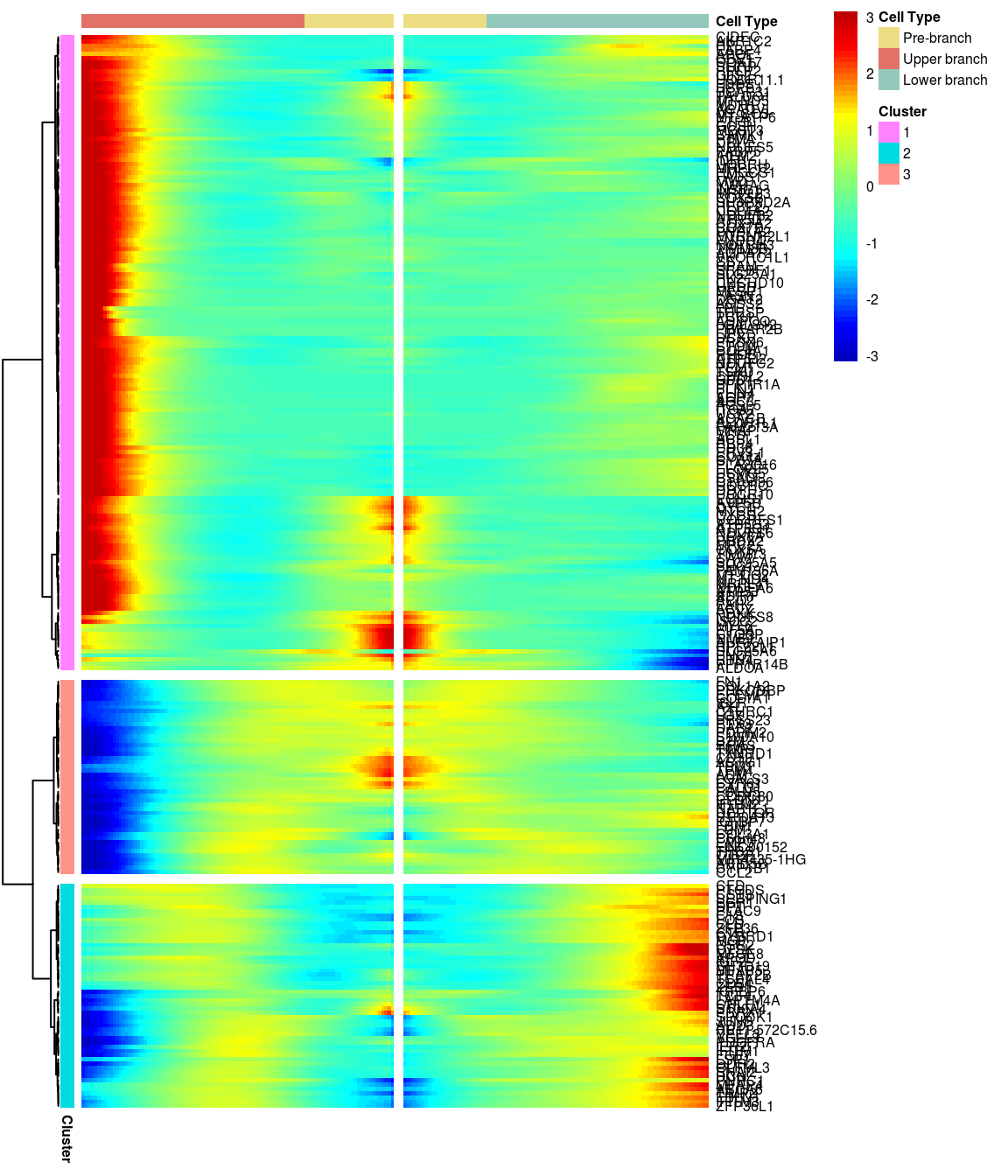 [1] “Total number of genes: 249” [1] “Nr of genes in cluster 1: 150” [1] “Nr of genes in cluster 2: 53” [1] “Nr of genes in cluster 3: 46”
BEAM heatmap: heatmap_logFC0.4_ncluster4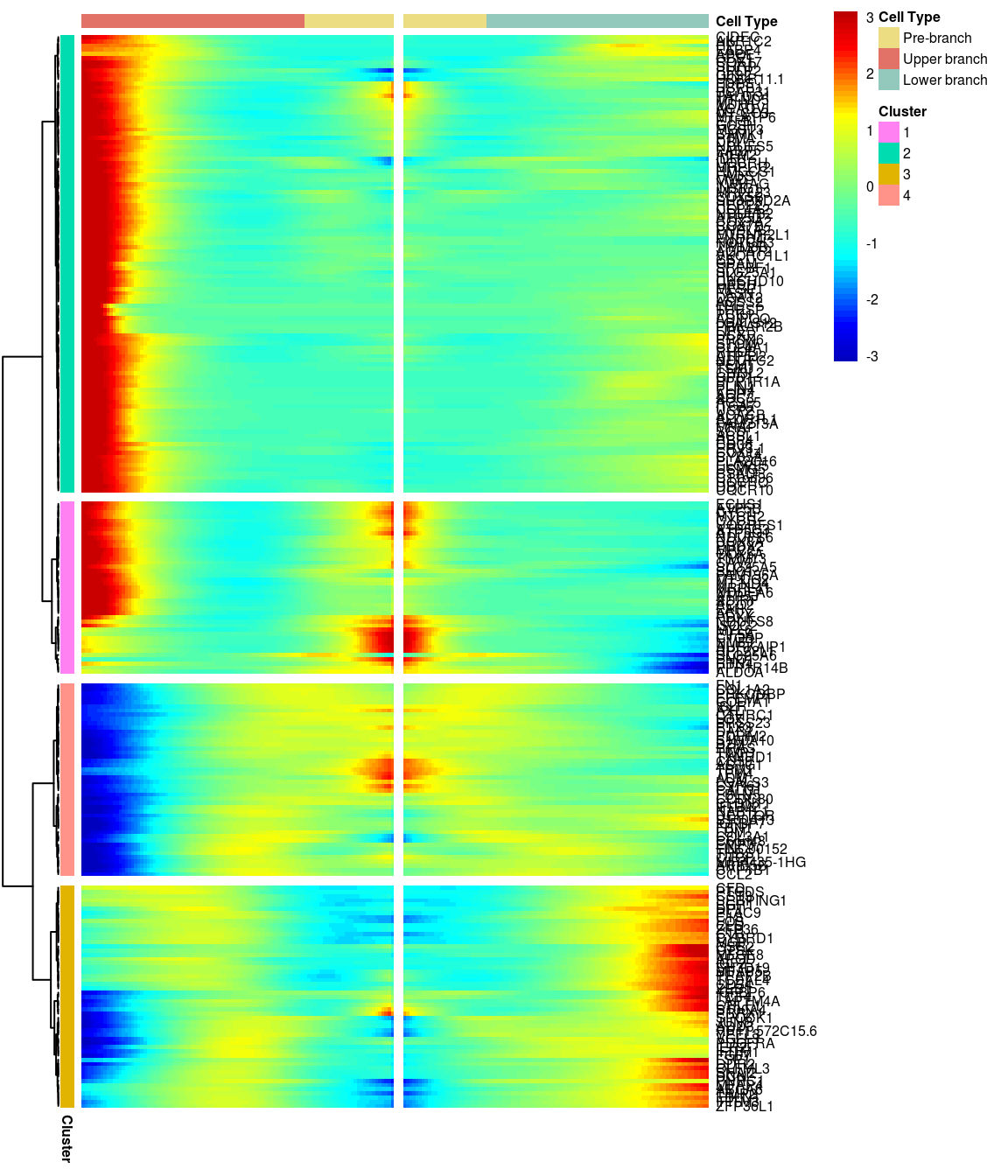 [1] “Total number of genes: 249” [1] “Nr of genes in cluster 1: 41” [1] “Nr of genes in cluster 2: 109” [1] “Nr of genes in cluster 3: 53” [1] “Nr of genes in cluster 4: 46”
BEAM heatmap: heatmap_logFC0.4_ncluster5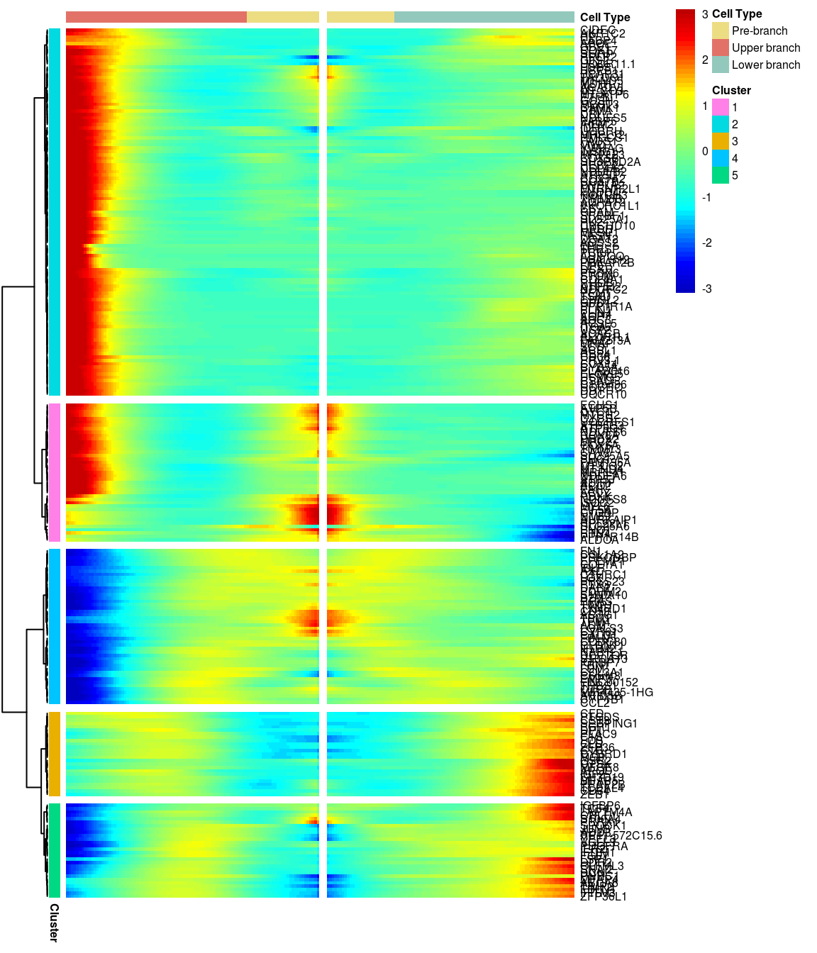 [1] “Total number of genes: 249” [1] “Nr of genes in cluster 1: 41” [1] “Nr of genes in cluster 2: 109” [1] “Nr of genes in cluster 3: 25” [1] “Nr of genes in cluster 4: 46” [1] “Nr of genes in cluster 5: 28”
BEAM heatmap: heatmap_logFC0.4_ncluster6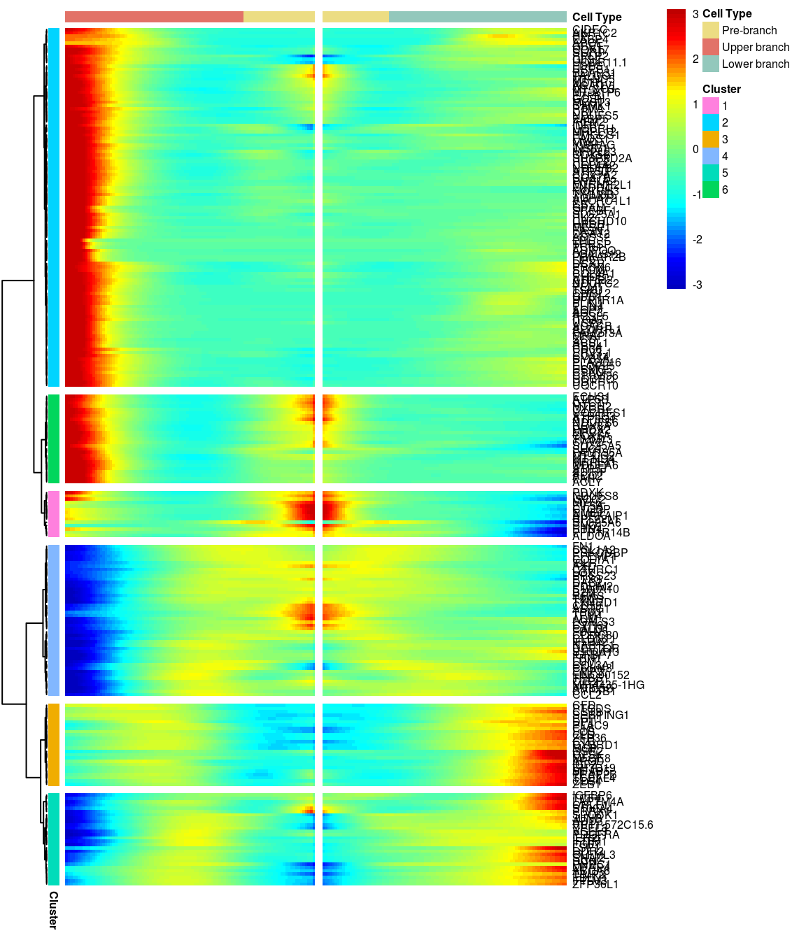 [1] “Total number of genes: 249” [1] “Nr of genes in cluster 1: 14” [1] “Nr of genes in cluster 2: 109” [1] “Nr of genes in cluster 3: 25” [1] “Nr of genes in cluster 4: 46” [1] “Nr of genes in cluster 5: 28” [1] “Nr of genes in cluster 6: 27”
BEAM heatmap: heatmap_logFC0.4_ncluster7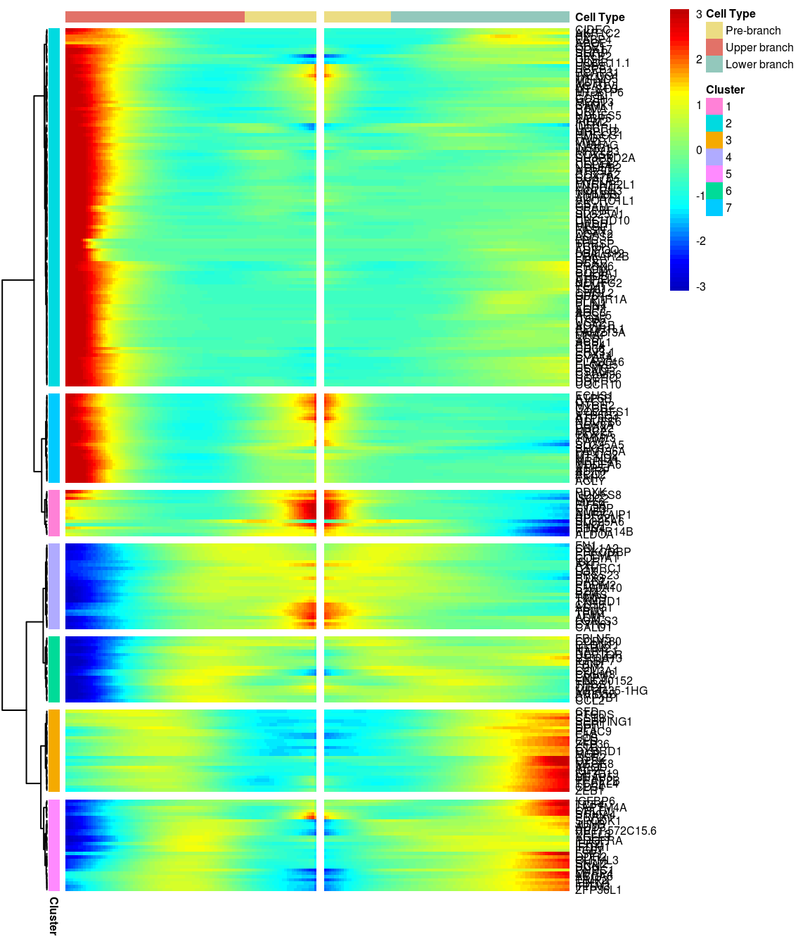 [1] “Total number of genes: 249” [1] “Nr of genes in cluster 1: 14” [1] “Nr of genes in cluster 2: 109” [1] “Nr of genes in cluster 3: 25” [1] “Nr of genes in cluster 4: 26” [1] “Nr of genes in cluster 5: 28” [1] “Nr of genes in cluster 6: 20” [1] “Nr of genes in cluster 7: 27”
BEAM heatmap: heatmap_logFC0.4_ncluster8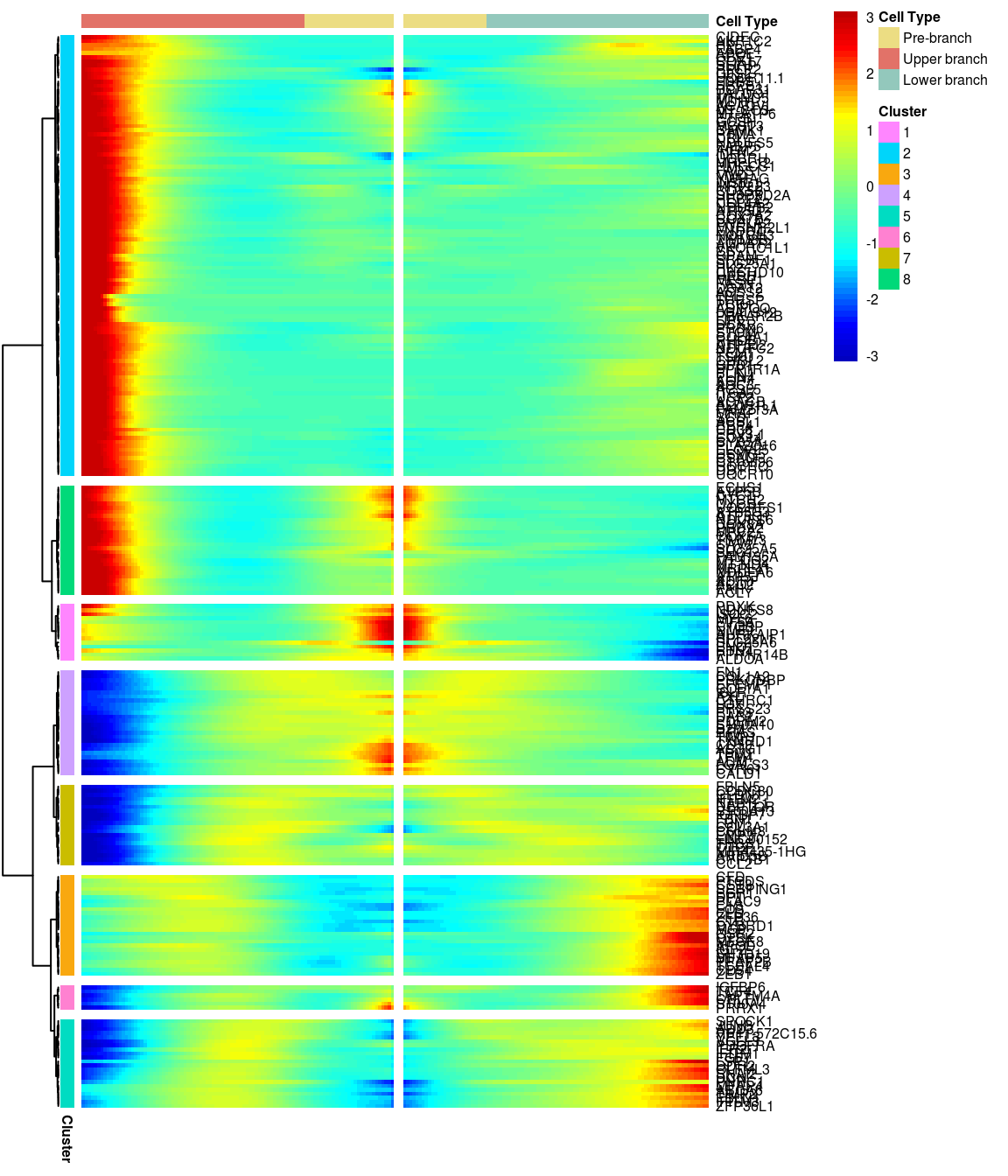 [1] “Total number of genes: 249” [1] “Nr of genes in cluster 1: 14” [1] “Nr of genes in cluster 2: 109” [1] “Nr of genes in cluster 3: 25” [1] “Nr of genes in cluster 4: 26” [1] “Nr of genes in cluster 5: 22” [1] “Nr of genes in cluster 6: 6” [1] “Nr of genes in cluster 7: 20” [1] “Nr of genes in cluster 8: 27”
BEAM heatmap: heatmap_logFC0.5_ncluster3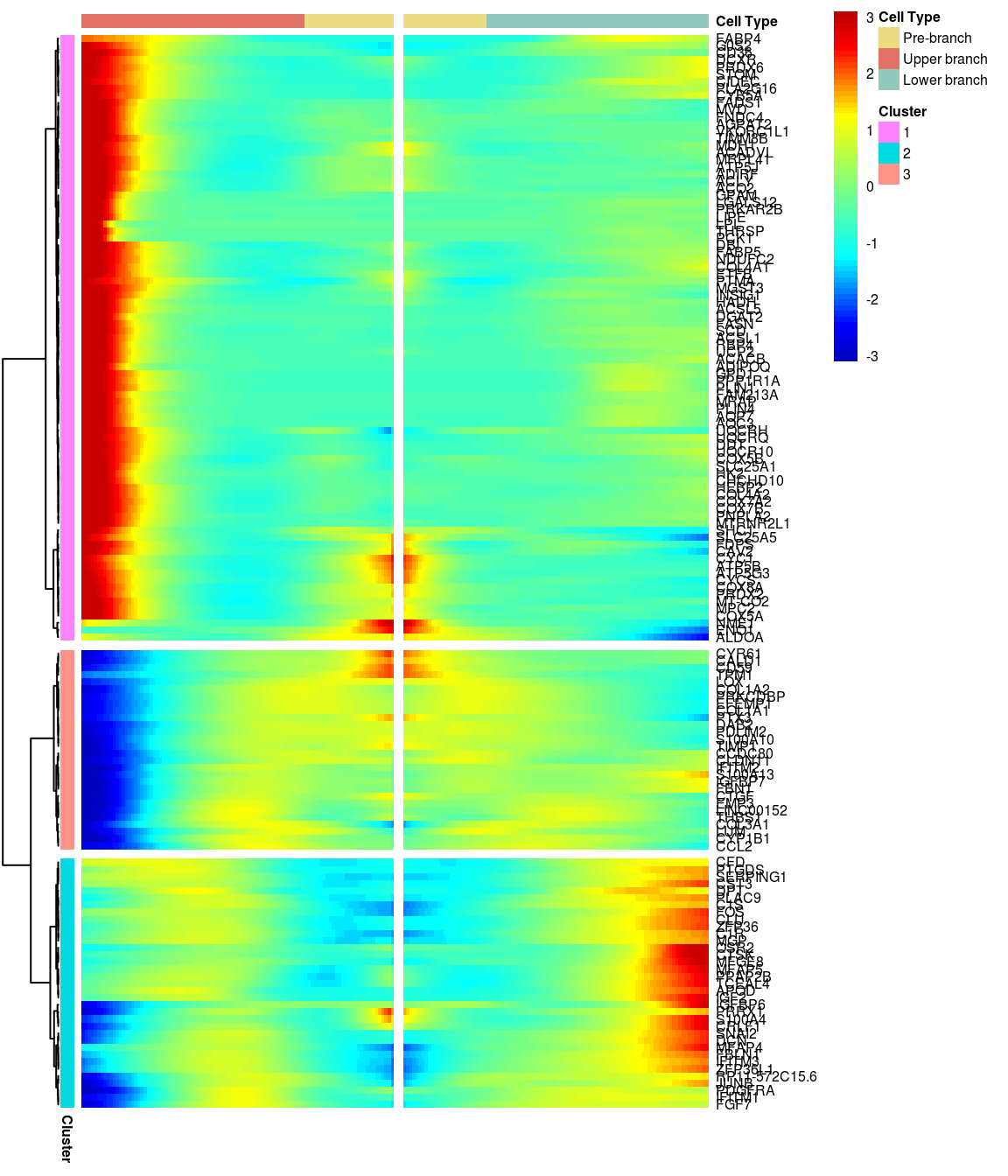 [1] “Total number of genes: 148” [1] “Nr of genes in cluster 1: 85” [1] “Nr of genes in cluster 2: 35” [1] “Nr of genes in cluster 3: 28”
BEAM heatmap: heatmap_logFC0.5_ncluster4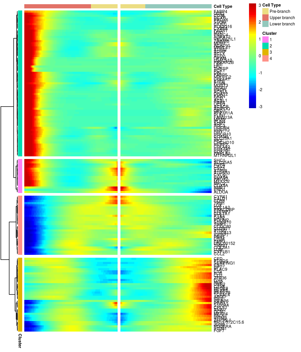 [1] “Total number of genes: 148” [1] “Nr of genes in cluster 1: 16” [1] “Nr of genes in cluster 2: 69” [1] “Nr of genes in cluster 3: 35” [1] “Nr of genes in cluster 4: 28”
BEAM heatmap: heatmap_logFC0.5_ncluster5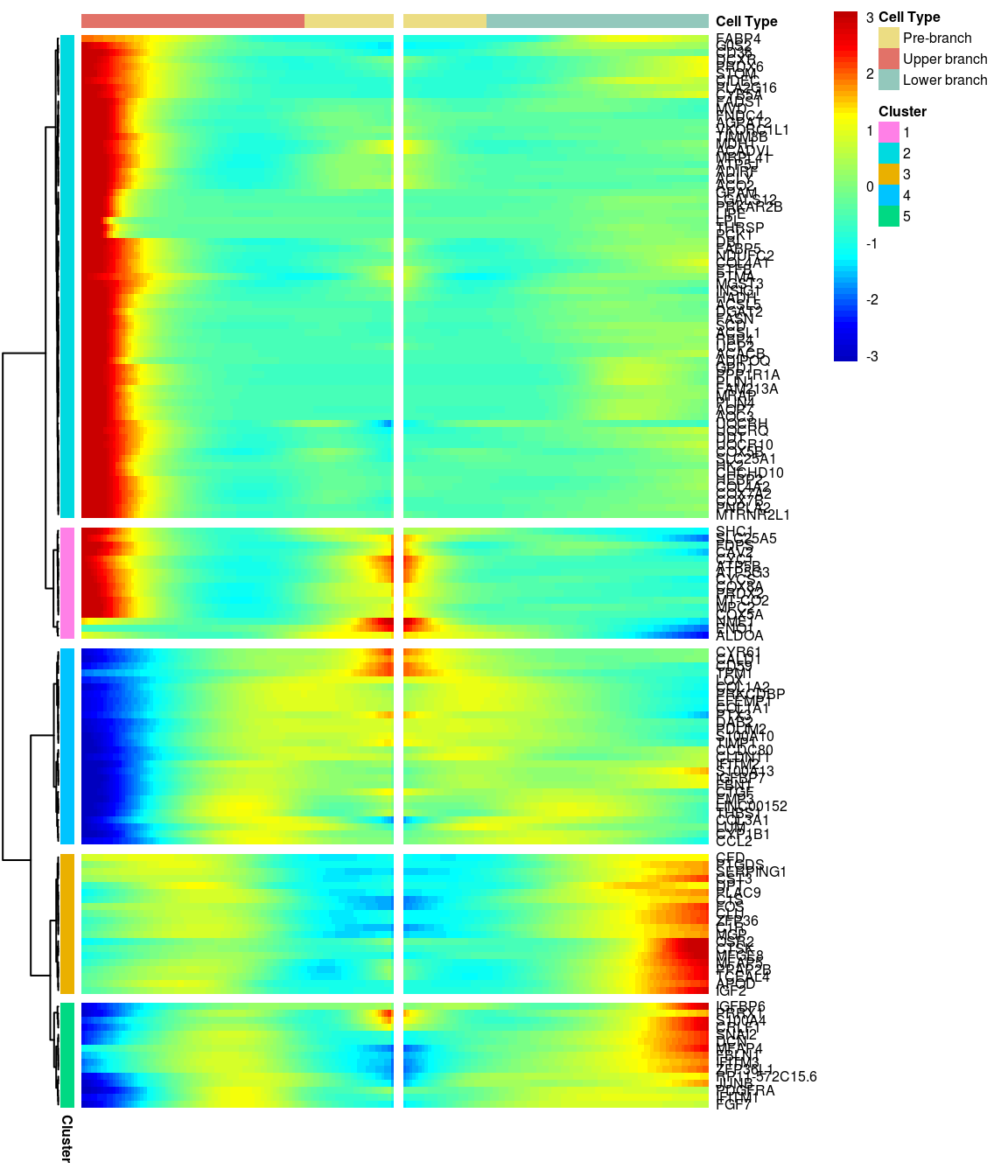 [1] “Total number of genes: 148” [1] “Nr of genes in cluster 1: 16” [1] “Nr of genes in cluster 2: 69” [1] “Nr of genes in cluster 3: 20” [1] “Nr of genes in cluster 4: 28” [1] “Nr of genes in cluster 5: 15”
BEAM heatmap: heatmap_logFC0.5_ncluster6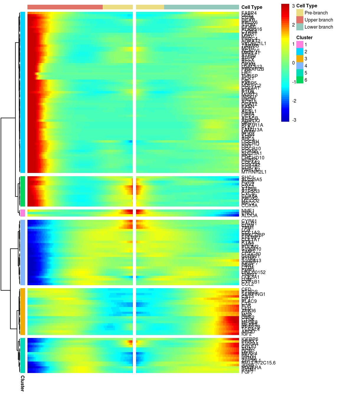 [1] “Total number of genes: 148” [1] “Nr of genes in cluster 1: 3” [1] “Nr of genes in cluster 2: 69” [1] “Nr of genes in cluster 3: 20” [1] “Nr of genes in cluster 4: 28” [1] “Nr of genes in cluster 5: 15” [1] “Nr of genes in cluster 6: 13”
BEAM heatmap: heatmap_logFC0.5_ncluster7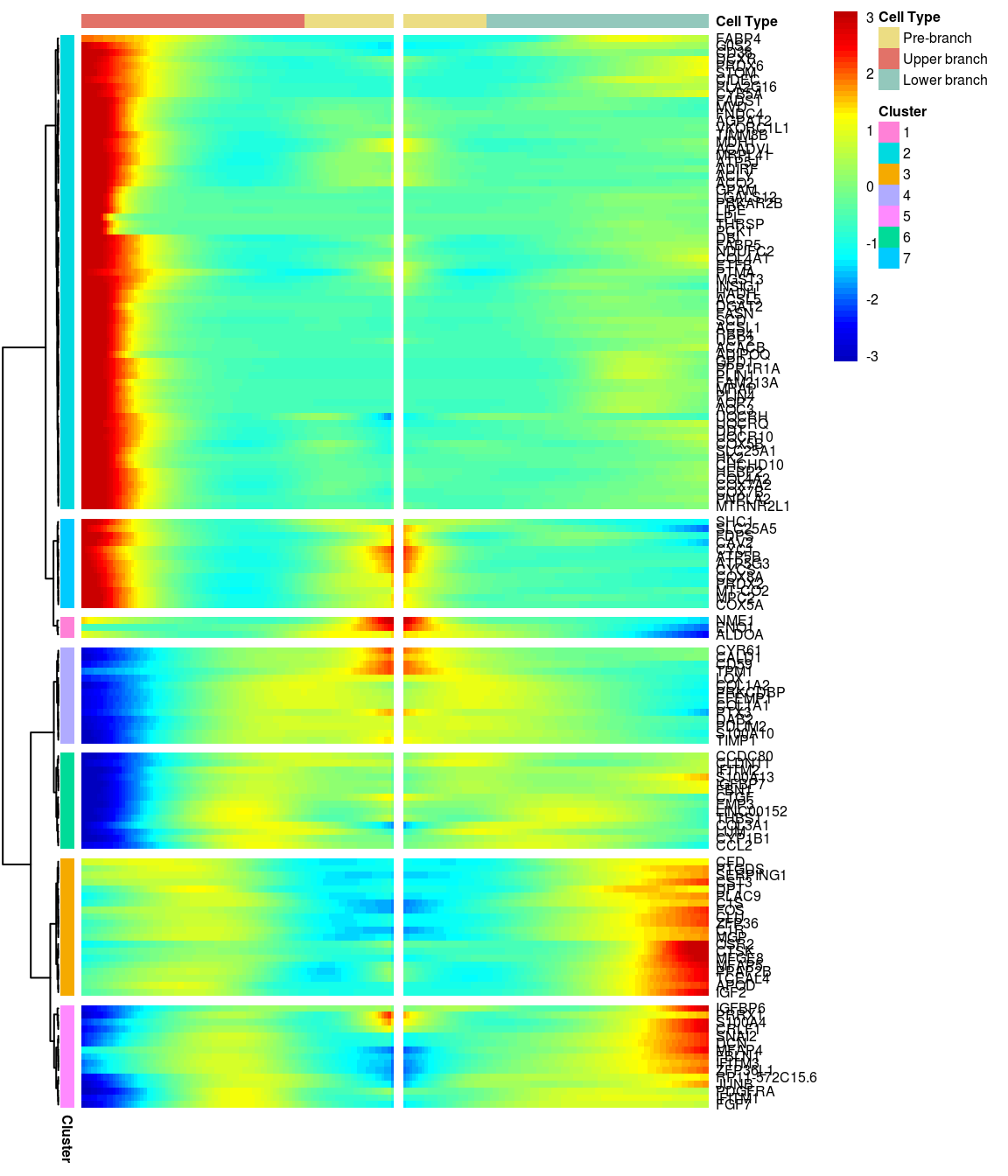 [1] “Total number of genes: 148” [1] “Nr of genes in cluster 1: 3” [1] “Nr of genes in cluster 2: 69” [1] “Nr of genes in cluster 3: 20” [1] “Nr of genes in cluster 4: 14” [1] “Nr of genes in cluster 5: 15” [1] “Nr of genes in cluster 6: 14” [1] “Nr of genes in cluster 7: 13”
BEAM heatmap: heatmap_logFC0.5_ncluster8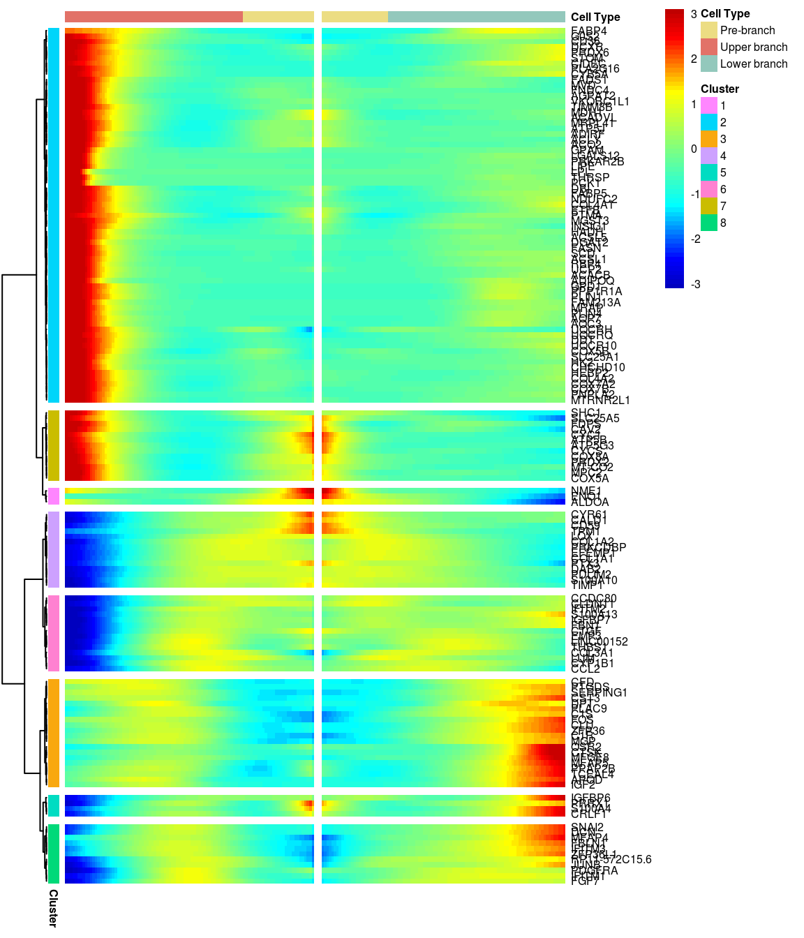 [1] “Total number of genes: 148” [1] “Nr of genes in cluster 1: 3” [1] “Nr of genes in cluster 2: 69” [1] “Nr of genes in cluster 3: 20” [1] “Nr of genes in cluster 4: 14” [1] “Nr of genes in cluster 5: 4” [1] “Nr of genes in cluster 6: 14” [1] “Nr of genes in cluster 7: 13” [1] “Nr of genes in cluster 8: 11”
BEAM heatmap: heatmap_logFC0.3_ncluster6_filtered_genes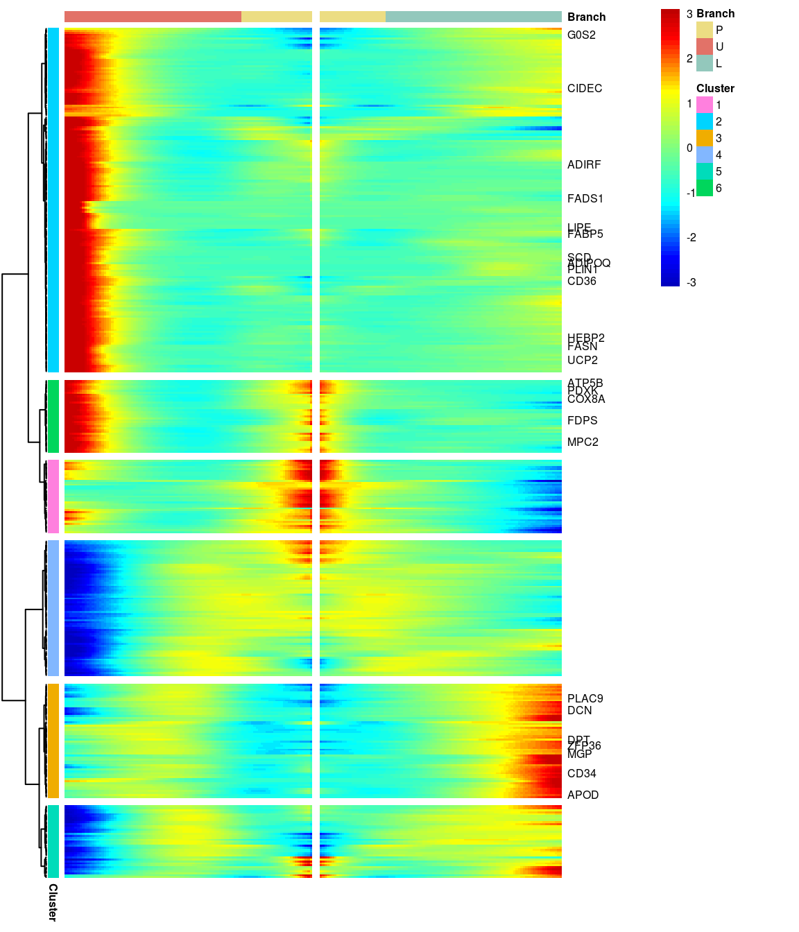 [1] “Total number of genes: 413” [1] “Nr of genes in cluster 1: 37” [1] “Nr of genes in cluster 2: 175” [1] “Nr of genes in cluster 3: 58” [1] “Nr of genes in cluster 4: 69” [1] “Nr of genes in cluster 5: 37” [1] “Nr of genes in cluster 6: 37”
BEAM heatmap: heatmap_logFC0.3_ncluster6_filtered_genes_OLD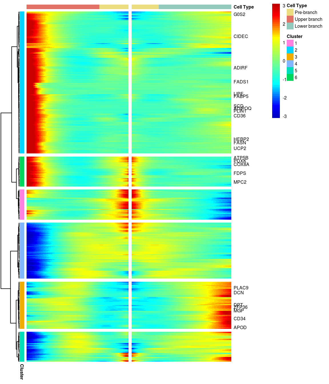 [1] “Total number of genes: 413” [1] “Nr of genes in cluster 1: 37” [1] “Nr of genes in cluster 2: 175” [1] “Nr of genes in cluster 3: 58” [1] “Nr of genes in cluster 4: 69” [1] “Nr of genes in cluster 5: 37” [1] “Nr of genes in cluster 6: 37”
sessionInfo()R version 3.5.3 (2019-03-11)
Platform: x86_64-pc-linux-gnu (64-bit)
Running under: Storage
Matrix products: default
BLAS/LAPACK: /usr/lib64/libopenblas-r0.3.3.so
locale:
[1] LC_CTYPE=en_US.UTF-8 LC_NUMERIC=C
[3] LC_TIME=en_US.UTF-8 LC_COLLATE=en_US.UTF-8
[5] LC_MONETARY=en_US.UTF-8 LC_MESSAGES=en_US.UTF-8
[7] LC_PAPER=en_US.UTF-8 LC_NAME=C
[9] LC_ADDRESS=C LC_TELEPHONE=C
[11] LC_MEASUREMENT=en_US.UTF-8 LC_IDENTIFICATION=C
attached base packages:
[1] splines stats4 parallel stats graphics grDevices utils
[8] datasets methods base
other attached packages:
[1] kableExtra_1.1.0 dplyr_0.8.0.1 gtools_3.8.1
[4] knitr_1.22 pheatmap_1.0.12 monocle_2.8.0
[7] DDRTree_0.1.5 irlba_2.3.3 VGAM_1.1-1
[10] Biobase_2.42.0 BiocGenerics_0.28.0 Seurat_2.3.4
[13] Matrix_1.2-17 cowplot_0.9.4 ggplot2_3.1.0
loaded via a namespace (and not attached):
[1] snow_0.4-3 backports_1.1.3 Hmisc_4.2-0
[4] workflowr_1.2.0 plyr_1.8.4 igraph_1.2.4
[7] lazyeval_0.2.2 densityClust_0.3 fastICA_1.2-1
[10] digest_0.6.18 foreach_1.4.4 htmltools_0.3.6
[13] viridis_0.5.1 lars_1.2 gdata_2.18.0
[16] magrittr_1.5 checkmate_1.9.1 cluster_2.0.7-1
[19] mixtools_1.1.0 ROCR_1.0-7 limma_3.36.5
[22] readr_1.3.1 matrixStats_0.54.0 R.utils_2.8.0
[25] docopt_0.6.1 colorspace_1.4-1 rvest_0.3.3
[28] ggrepel_0.8.0 xfun_0.5 sparsesvd_0.1-4
[31] crayon_1.3.4 jsonlite_1.6 survival_2.43-3
[34] zoo_1.8-5 iterators_1.0.10 ape_5.3
[37] glue_1.3.1 gtable_0.3.0 webshot_0.5.1
[40] kernlab_0.9-27 prabclus_2.2-7 DEoptimR_1.0-8
[43] scales_1.0.0 mvtnorm_1.0-10 bibtex_0.4.2
[46] Rcpp_1.0.1 metap_1.1 dtw_1.20-1
[49] viridisLite_0.3.0 htmlTable_1.13.1 reticulate_1.11.1
[52] foreign_0.8-71 bit_1.1-14 proxy_0.4-23
[55] mclust_5.4.3 SDMTools_1.1-221 Formula_1.2-3
[58] tsne_0.1-3 htmlwidgets_1.3 httr_1.4.0
[61] FNN_1.1.3 gplots_3.0.1.1 RColorBrewer_1.1-2
[64] fpc_2.1-11.1 acepack_1.4.1 modeltools_0.2-22
[67] ica_1.0-2 pkgconfig_2.0.2 R.methodsS3_1.7.1
[70] flexmix_2.3-15 nnet_7.3-12 labeling_0.3
[73] tidyselect_0.2.5 rlang_0.3.2 reshape2_1.4.3
[76] munsell_0.5.0 tools_3.5.3 ggridges_0.5.1
[79] evaluate_0.13 stringr_1.4.0 yaml_2.2.0
[82] npsurv_0.4-0 bit64_0.9-7 fs_1.2.7
[85] fitdistrplus_1.0-14 robustbase_0.93-4 caTools_1.17.1.2
[88] purrr_0.3.2 RANN_2.6.1 pbapply_1.4-0
[91] nlme_3.1-137 whisker_0.3-2 slam_0.1-45
[94] R.oo_1.22.0 xml2_1.2.0 hdf5r_1.1.1
[97] compiler_3.5.3 rstudioapi_0.10 png_0.1-7
[100] lsei_1.2-0 tibble_2.1.1 stringi_1.4.3
[103] highr_0.8 lattice_0.20-38 trimcluster_0.1-2.1
[106] HSMMSingleCell_0.114.0 pillar_1.3.1 combinat_0.0-8
[109] Rdpack_0.10-1 lmtest_0.9-36 data.table_1.12.0
[112] bitops_1.0-6 gbRd_0.4-11 R6_2.4.0
[115] latticeExtra_0.6-28 KernSmooth_2.23-15 gridExtra_2.3
[118] codetools_0.2-16 MASS_7.3-51.1 assertthat_0.2.1
[121] rprojroot_1.3-2 withr_2.1.2 qlcMatrix_0.9.7
[124] hms_0.4.2 diptest_0.75-7 doSNOW_1.0.16
[127] grid_3.5.3 rpart_4.1-13 tidyr_0.8.3
[130] class_7.3-15 rmarkdown_1.12 segmented_0.5-3.0
[133] Rtsne_0.15 git2r_0.25.2 base64enc_0.1-3